This test problem explains and demonstrates the application of temperature gradient to bridge objects. To summarize the process, temperature gradient is specified and applied to the transformed section, axial force (P) and moment (M3) are calculated, then an equivalent constant + linear temperature distribution is applied over the depth.
This process enables the correct calculation of overall cross-sectional force and moment. Nodal application of actual temperatures induced by the temperature distribution specified would yield incorrect net fore and moment without the cross section being finely discretized.
On this page:Procedure
The stress distribution of a temperature gradient is calculated as E α T. Users may analytically solve for axial force (P) by integrating this expression over the section, accounting for the web and flange areas. To solve for M3, integrate the moment of stresses about the neutral axis.
CSI
Software derives temperature-gradient response by following these formulations. First, the software assumes a linear gradient with two unknowns, including neutral-axis value and gradient slope. Integration procedures yield a set of polynomial expression for P and M3. Simultaneous solution then yields exact expressions for axial force and moment.
Examples
The following two examples demonstrate temperature-gradient application. Screenshots and attached hand calculations illustrate the procedure.
Example 1 - bridge-modeler model
Please note that the hand calculations attached provide additional details.
A single-span concrete-box bridge, fixed at both abutments, is created using the bridge modeler. The linked bridge object is updated as a solid model. Loading from temperature gradient is defined as shown in Figure 1:
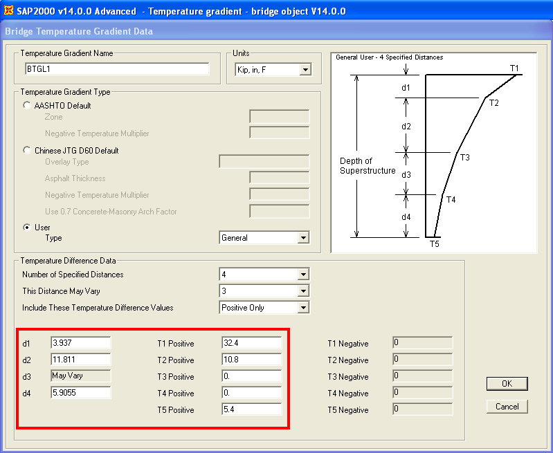
Figure 1 - Temperature-gradient loading
As mentioned earlier, an equivalent constant + linear temperature gradient generates the temperature load for a solid model. This procedure correlates precisely with the attached hand calculations , as shown in Figure 2:

Figure 2 - Temperature-gradient loading on solid elements
For bridge response, loading from the temperature gradient induces a moment of 2568 kip-ft, which closely correlates with the hand calculated moment of 2669 kip-ft. Software output is shown in Figure 3:

Figure 3 - Moment induced by temperature gradient
Example 2 - single frame-element model
Please note that the hand calculations attached provide additional details.
For example 2, a single, beam frame element is fixed at both ends and manually loaded with the constant + linear temperature gradient. Element cross section is defined to match those properties of the entire bridge deck section from example 1. The temperature-gradient loading creates a moment of 2668 kip-ft, nearly identical to the hand-calculated moment of 2669 kip-ft. Software output is shown in Figure 4:
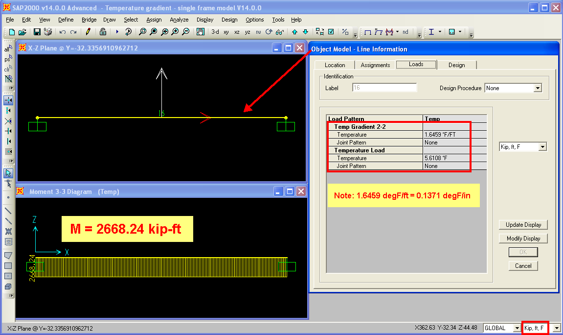
Figure 4 - Temperature-gradient on the frame-element model
Attachments
- Hand calculations (PDF file)
- SAP2000 models (zipped SDB files) - example 1, bridge-modeler model and example 2, single frame-element model